This is a notebook from a presentation I recently gave to the UofT scientific coding group. There was a good turnout and it gave me good experience for this sort of coding walkthrough as a teaching experience.
You can check out the screencast on youtube.
Objectives
- Read tabular data into an IPython notebook
- Access columns of the data
- Isolate subsets of the data
- Generate plots based on subsetted data
Resources
Pandas has lots of great documentation, tutorials and walkthroughs.
This tutorial was based largely off of a SWC inspired lesson by Nancy Soontiens.
I adapted other parts from a great tutorial by Greg Reda.
More can also be found in the pandas documentation.
A great youtube walkthrough from PyCon 2015:
I've also found a recent set of helpful blogposts for intermediate and advanced users.
Working with dataframes
import pandas as pd
import numpy as np
import matplotlib.pyplot as plt
pandas introduces two new data structures to Python - Series and DataFrame, both of which are built on top of NumPy.
We can load in a tabular data set as a dataframe in a number of different ways.
df = pd.read_table('./gapminderDataFiveYear.txt')
df
| country | year | pop | continent | lifeExp | gdpPercap | |
|---|---|---|---|---|---|---|
| 0 | Afghanistan | 1952 | 8425333 | Asia | 28.801 | 779.445314 |
| 1 | Afghanistan | 1957 | 9240934 | Asia | 30.332 | 820.853030 |
| 2 | Afghanistan | 1962 | 10267083 | Asia | 31.997 | 853.100710 |
| 3 | Afghanistan | 1967 | 11537966 | Asia | 34.020 | 836.197138 |
| 4 | Afghanistan | 1972 | 13079460 | Asia | 36.088 | 739.981106 |
| 5 | Afghanistan | 1977 | 14880372 | Asia | 38.438 | 786.113360 |
| 6 | Afghanistan | 1982 | 12881816 | Asia | 39.854 | 978.011439 |
| 7 | Afghanistan | 1987 | 13867957 | Asia | 40.822 | 852.395945 |
| 8 | Afghanistan | 1992 | 16317921 | Asia | 41.674 | 649.341395 |
| 9 | Afghanistan | 1997 | 22227415 | Asia | 41.763 | 635.341351 |
| 10 | Afghanistan | 2002 | 25268405 | Asia | 42.129 | 726.734055 |
| 11 | Afghanistan | 2007 | 31889923 | Asia | 43.828 | 974.580338 |
| 12 | Albania | 1952 | 1282697 | Europe | 55.230 | 1601.056136 |
| 13 | Albania | 1957 | 1476505 | Europe | 59.280 | 1942.284244 |
| 14 | Albania | 1962 | 1728137 | Europe | 64.820 | 2312.888958 |
| 15 | Albania | 1967 | 1984060 | Europe | 66.220 | 2760.196931 |
| 16 | Albania | 1972 | 2263554 | Europe | 67.690 | 3313.422188 |
| 17 | Albania | 1977 | 2509048 | Europe | 68.930 | 3533.003910 |
| 18 | Albania | 1982 | 2780097 | Europe | 70.420 | 3630.880722 |
| 19 | Albania | 1987 | 3075321 | Europe | 72.000 | 3738.932735 |
| 20 | Albania | 1992 | 3326498 | Europe | 71.581 | 2497.437901 |
| 21 | Albania | 1997 | 3428038 | Europe | 72.950 | 3193.054604 |
| 22 | Albania | 2002 | 3508512 | Europe | 75.651 | 4604.211737 |
| 23 | Albania | 2007 | 3600523 | Europe | 76.423 | 5937.029526 |
| 24 | Algeria | 1952 | 9279525 | Africa | 43.077 | 2449.008185 |
| 25 | Algeria | 1957 | 10270856 | Africa | 45.685 | 3013.976023 |
| 26 | Algeria | 1962 | 11000948 | Africa | 48.303 | 2550.816880 |
| 27 | Algeria | 1967 | 12760499 | Africa | 51.407 | 3246.991771 |
| 28 | Algeria | 1972 | 14760787 | Africa | 54.518 | 4182.663766 |
| 29 | Algeria | 1977 | 17152804 | Africa | 58.014 | 4910.416756 |
| ... | ... | ... | ... | ... | ... | ... |
| 1674 | Yemen, Rep. | 1982 | 9657618 | Asia | 49.113 | 1977.557010 |
| 1675 | Yemen, Rep. | 1987 | 11219340 | Asia | 52.922 | 1971.741538 |
| 1676 | Yemen, Rep. | 1992 | 13367997 | Asia | 55.599 | 1879.496673 |
| 1677 | Yemen, Rep. | 1997 | 15826497 | Asia | 58.020 | 2117.484526 |
| 1678 | Yemen, Rep. | 2002 | 18701257 | Asia | 60.308 | 2234.820827 |
| 1679 | Yemen, Rep. | 2007 | 22211743 | Asia | 62.698 | 2280.769906 |
| 1680 | Zambia | 1952 | 2672000 | Africa | 42.038 | 1147.388831 |
| 1681 | Zambia | 1957 | 3016000 | Africa | 44.077 | 1311.956766 |
| 1682 | Zambia | 1962 | 3421000 | Africa | 46.023 | 1452.725766 |
| 1683 | Zambia | 1967 | 3900000 | Africa | 47.768 | 1777.077318 |
| 1684 | Zambia | 1972 | 4506497 | Africa | 50.107 | 1773.498265 |
| 1685 | Zambia | 1977 | 5216550 | Africa | 51.386 | 1588.688299 |
| 1686 | Zambia | 1982 | 6100407 | Africa | 51.821 | 1408.678565 |
| 1687 | Zambia | 1987 | 7272406 | Africa | 50.821 | 1213.315116 |
| 1688 | Zambia | 1992 | 8381163 | Africa | 46.100 | 1210.884633 |
| 1689 | Zambia | 1997 | 9417789 | Africa | 40.238 | 1071.353818 |
| 1690 | Zambia | 2002 | 10595811 | Africa | 39.193 | 1071.613938 |
| 1691 | Zambia | 2007 | 11746035 | Africa | 42.384 | 1271.211593 |
| 1692 | Zimbabwe | 1952 | 3080907 | Africa | 48.451 | 406.884115 |
| 1693 | Zimbabwe | 1957 | 3646340 | Africa | 50.469 | 518.764268 |
| 1694 | Zimbabwe | 1962 | 4277736 | Africa | 52.358 | 527.272182 |
| 1695 | Zimbabwe | 1967 | 4995432 | Africa | 53.995 | 569.795071 |
| 1696 | Zimbabwe | 1972 | 5861135 | Africa | 55.635 | 799.362176 |
| 1697 | Zimbabwe | 1977 | 6642107 | Africa | 57.674 | 685.587682 |
| 1698 | Zimbabwe | 1982 | 7636524 | Africa | 60.363 | 788.855041 |
| 1699 | Zimbabwe | 1987 | 9216418 | Africa | 62.351 | 706.157306 |
| 1700 | Zimbabwe | 1992 | 10704340 | Africa | 60.377 | 693.420786 |
| 1701 | Zimbabwe | 1997 | 11404948 | Africa | 46.809 | 792.449960 |
| 1702 | Zimbabwe | 2002 | 11926563 | Africa | 39.989 | 672.038623 |
| 1703 | Zimbabwe | 2007 | 12311143 | Africa | 43.487 | 469.709298 |
1704 rows × 6 columns
type(df)
pandas.core.frame.DataFrame
df.shape
(1704, 6)
df.columns
Index(['country', 'year', 'pop', 'continent', 'lifeExp', 'gdpPercap'], dtype='object')
df.head()
| country | year | pop | continent | lifeExp | gdpPercap | |
|---|---|---|---|---|---|---|
| 0 | Afghanistan | 1952 | 8425333 | Asia | 28.801 | 779.445314 |
| 1 | Afghanistan | 1957 | 9240934 | Asia | 30.332 | 820.853030 |
| 2 | Afghanistan | 1962 | 10267083 | Asia | 31.997 | 853.100710 |
| 3 | Afghanistan | 1967 | 11537966 | Asia | 34.020 | 836.197138 |
| 4 | Afghanistan | 1972 | 13079460 | Asia | 36.088 | 739.981106 |
df.head(6)
| country | year | pop | continent | lifeExp | gdpPercap | |
|---|---|---|---|---|---|---|
| 0 | Afghanistan | 1952 | 8425333 | Asia | 28.801 | 779.445314 |
| 1 | Afghanistan | 1957 | 9240934 | Asia | 30.332 | 820.853030 |
| 2 | Afghanistan | 1962 | 10267083 | Asia | 31.997 | 853.100710 |
| 3 | Afghanistan | 1967 | 11537966 | Asia | 34.020 | 836.197138 |
| 4 | Afghanistan | 1972 | 13079460 | Asia | 36.088 | 739.981106 |
| 5 | Afghanistan | 1977 | 14880372 | Asia | 38.438 | 786.113360 |
df.tail()
| country | year | pop | continent | lifeExp | gdpPercap | |
|---|---|---|---|---|---|---|
| 1699 | Zimbabwe | 1987 | 9216418 | Africa | 62.351 | 706.157306 |
| 1700 | Zimbabwe | 1992 | 10704340 | Africa | 60.377 | 693.420786 |
| 1701 | Zimbabwe | 1997 | 11404948 | Africa | 46.809 | 792.449960 |
| 1702 | Zimbabwe | 2002 | 11926563 | Africa | 39.989 | 672.038623 |
| 1703 | Zimbabwe | 2007 | 12311143 | Africa | 43.487 | 469.709298 |
df.info()
<class 'pandas.core.frame.DataFrame'>
Int64Index: 1704 entries, 0 to 1703
Data columns (total 6 columns):
country      1704 non-null object
year         1704 non-null int64
pop          1704 non-null float64
continent    1704 non-null object
lifeExp      1704 non-null float64
gdpPercap    1704 non-null float64
dtypes: float64(3), int64(1), object(2)
memory usage: 93.2+ KB
df.dtypes
country       object
year           int64
pop          float64
continent     object
lifeExp      float64
gdpPercap    float64
dtype: object
Get summary statistics for the numeric columns with the describe() method
df.describe()
| year | pop | lifeExp | gdpPercap | |
|---|---|---|---|---|
| count | 1704.00000 | 1.704000e+03 | 1704.000000 | 1704.000000 |
| mean | 1979.50000 | 2.960121e+07 | 59.474439 | 7215.327081 |
| std | 17.26533 | 1.061579e+08 | 12.917107 | 9857.454543 |
| min | 1952.00000 | 6.001100e+04 | 23.599000 | 241.165877 |
| 25% | 1965.75000 | 2.793664e+06 | 48.198000 | 1202.060309 |
| 50% | 1979.50000 | 7.023596e+06 | 60.712500 | 3531.846989 |
| 75% | 1993.25000 | 1.958522e+07 | 70.845500 | 9325.462346 |
| max | 2007.00000 | 1.318683e+09 | 82.603000 | 113523.132900 |
Data selection
Sometimes we need to look at only parts of the data. For example, we might want to look at the data for a particular country or in a particular year.
Selecting columns
#select multiple columns with a list of column names
col_list = ['year','lifeExp', 'country']
df[col_list]
| year | lifeExp | country | |
|---|---|---|---|
| 0 | 1952 | 28.801 | Afghanistan |
| 1 | 1957 | 30.332 | Afghanistan |
| 2 | 1962 | 31.997 | Afghanistan |
| 3 | 1967 | 34.020 | Afghanistan |
| 4 | 1972 | 36.088 | Afghanistan |
| 5 | 1977 | 38.438 | Afghanistan |
| 6 | 1982 | 39.854 | Afghanistan |
| 7 | 1987 | 40.822 | Afghanistan |
| 8 | 1992 | 41.674 | Afghanistan |
| 9 | 1997 | 41.763 | Afghanistan |
| 10 | 2002 | 42.129 | Afghanistan |
| 11 | 2007 | 43.828 | Afghanistan |
| 12 | 1952 | 55.230 | Albania |
| 13 | 1957 | 59.280 | Albania |
| 14 | 1962 | 64.820 | Albania |
| 15 | 1967 | 66.220 | Albania |
| 16 | 1972 | 67.690 | Albania |
| 17 | 1977 | 68.930 | Albania |
| 18 | 1982 | 70.420 | Albania |
| 19 | 1987 | 72.000 | Albania |
| 20 | 1992 | 71.581 | Albania |
| 21 | 1997 | 72.950 | Albania |
| 22 | 2002 | 75.651 | Albania |
| 23 | 2007 | 76.423 | Albania |
| 24 | 1952 | 43.077 | Algeria |
| 25 | 1957 | 45.685 | Algeria |
| 26 | 1962 | 48.303 | Algeria |
| 27 | 1967 | 51.407 | Algeria |
| 28 | 1972 | 54.518 | Algeria |
| 29 | 1977 | 58.014 | Algeria |
| ... | ... | ... | ... |
| 1674 | 1982 | 49.113 | Yemen, Rep. |
| 1675 | 1987 | 52.922 | Yemen, Rep. |
| 1676 | 1992 | 55.599 | Yemen, Rep. |
| 1677 | 1997 | 58.020 | Yemen, Rep. |
| 1678 | 2002 | 60.308 | Yemen, Rep. |
| 1679 | 2007 | 62.698 | Yemen, Rep. |
| 1680 | 1952 | 42.038 | Zambia |
| 1681 | 1957 | 44.077 | Zambia |
| 1682 | 1962 | 46.023 | Zambia |
| 1683 | 1967 | 47.768 | Zambia |
| 1684 | 1972 | 50.107 | Zambia |
| 1685 | 1977 | 51.386 | Zambia |
| 1686 | 1982 | 51.821 | Zambia |
| 1687 | 1987 | 50.821 | Zambia |
| 1688 | 1992 | 46.100 | Zambia |
| 1689 | 1997 | 40.238 | Zambia |
| 1690 | 2002 | 39.193 | Zambia |
| 1691 | 2007 | 42.384 | Zambia |
| 1692 | 1952 | 48.451 | Zimbabwe |
| 1693 | 1957 | 50.469 | Zimbabwe |
| 1694 | 1962 | 52.358 | Zimbabwe |
| 1695 | 1967 | 53.995 | Zimbabwe |
| 1696 | 1972 | 55.635 | Zimbabwe |
| 1697 | 1977 | 57.674 | Zimbabwe |
| 1698 | 1982 | 60.363 | Zimbabwe |
| 1699 | 1987 | 62.351 | Zimbabwe |
| 1700 | 1992 | 60.377 | Zimbabwe |
| 1701 | 1997 | 46.809 | Zimbabwe |
| 1702 | 2002 | 39.989 | Zimbabwe |
| 1703 | 2007 | 43.487 | Zimbabwe |
1704 rows × 3 columns
#alternative selection with dot notation won't work if column names have spaces, uncommon characters or leading numbers
df.lifeExp
0       28.801
1       30.332
2       31.997
3       34.020
4       36.088
5       38.438
6       39.854
7       40.822
8       41.674
9       41.763
10      42.129
11      43.828
12      55.230
13      59.280
14      64.820
15      66.220
16      67.690
17      68.930
18      70.420
19      72.000
20      71.581
21      72.950
22      75.651
23      76.423
24      43.077
25      45.685
26      48.303
27      51.407
28      54.518
29      58.014
         ...
1674    49.113
1675    52.922
1676    55.599
1677    58.020
1678    60.308
1679    62.698
1680    42.038
1681    44.077
1682    46.023
1683    47.768
1684    50.107
1685    51.386
1686    51.821
1687    50.821
1688    46.100
1689    40.238
1690    39.193
1691    42.384
1692    48.451
1693    50.469
1694    52.358
1695    53.995
1696    55.635
1697    57.674
1698    60.363
1699    62.351
1700    60.377
1701    46.809
1702    39.989
1703    43.487
Name: lifeExp, dtype: float64
#using describe() on a categorical column
df[['country', 'continent']].describe()
| country | continent | |
|---|---|---|
| count | 1704 | 1704 |
| unique | 142 | 5 |
| top | Guatemala | Africa |
| freq | 12 | 624 |
Selecting rows
#by index location
df.iloc[[1000]]
| country | year | pop | continent | lifeExp | gdpPercap | |
|---|---|---|---|---|---|---|
| 1000 | Mongolia | 1972 | 1320500 | Asia | 53.754 | 1421.741975 |
#you can provide a list of index values to select
df.iloc[[0,5,10]]
| country | year | pop | continent | lifeExp | gdpPercap | |
|---|---|---|---|---|---|---|
| 0 | Afghanistan | 1952 | 8425333 | Asia | 28.801 | 779.445314 |
| 5 | Afghanistan | 1977 | 14880372 | Asia | 38.438 | 786.113360 |
| 10 | Afghanistan | 2002 | 25268405 | Asia | 42.129 | 726.734055 |
#or select with the slice notation
df[0:5]
| country | year | pop | continent | lifeExp | gdpPercap | |
|---|---|---|---|---|---|---|
| 0 | Afghanistan | 1952 | 8425333 | Asia | 28.801 | 779.445314 |
| 1 | Afghanistan | 1957 | 9240934 | Asia | 30.332 | 820.853030 |
| 2 | Afghanistan | 1962 | 10267083 | Asia | 31.997 | 853.100710 |
| 3 | Afghanistan | 1967 | 11537966 | Asia | 34.020 | 836.197138 |
| 4 | Afghanistan | 1972 | 13079460 | Asia | 36.088 | 739.981106 |
#select by index label
#would require named index
country_index = df.set_index(['continent','country'])
country_index
| year | pop | lifeExp | gdpPercap | ||
|---|---|---|---|---|---|
| continent | country | ||||
| Asia | Afghanistan | 1952 | 8425333 | 28.801 | 779.445314 |
| Afghanistan | 1957 | 9240934 | 30.332 | 820.853030 | |
| Afghanistan | 1962 | 10267083 | 31.997 | 853.100710 | |
| Afghanistan | 1967 | 11537966 | 34.020 | 836.197138 | |
| Afghanistan | 1972 | 13079460 | 36.088 | 739.981106 | |
| Afghanistan | 1977 | 14880372 | 38.438 | 786.113360 | |
| Afghanistan | 1982 | 12881816 | 39.854 | 978.011439 | |
| Afghanistan | 1987 | 13867957 | 40.822 | 852.395945 | |
| Afghanistan | 1992 | 16317921 | 41.674 | 649.341395 | |
| Afghanistan | 1997 | 22227415 | 41.763 | 635.341351 | |
| Afghanistan | 2002 | 25268405 | 42.129 | 726.734055 | |
| Afghanistan | 2007 | 31889923 | 43.828 | 974.580338 | |
| Europe | Albania | 1952 | 1282697 | 55.230 | 1601.056136 |
| Albania | 1957 | 1476505 | 59.280 | 1942.284244 | |
| Albania | 1962 | 1728137 | 64.820 | 2312.888958 | |
| Albania | 1967 | 1984060 | 66.220 | 2760.196931 | |
| Albania | 1972 | 2263554 | 67.690 | 3313.422188 | |
| Albania | 1977 | 2509048 | 68.930 | 3533.003910 | |
| Albania | 1982 | 2780097 | 70.420 | 3630.880722 | |
| Albania | 1987 | 3075321 | 72.000 | 3738.932735 | |
| Albania | 1992 | 3326498 | 71.581 | 2497.437901 | |
| Albania | 1997 | 3428038 | 72.950 | 3193.054604 | |
| Albania | 2002 | 3508512 | 75.651 | 4604.211737 | |
| Albania | 2007 | 3600523 | 76.423 | 5937.029526 | |
| Africa | Algeria | 1952 | 9279525 | 43.077 | 2449.008185 |
| Algeria | 1957 | 10270856 | 45.685 | 3013.976023 | |
| Algeria | 1962 | 11000948 | 48.303 | 2550.816880 | |
| Algeria | 1967 | 12760499 | 51.407 | 3246.991771 | |
| Algeria | 1972 | 14760787 | 54.518 | 4182.663766 | |
| Algeria | 1977 | 17152804 | 58.014 | 4910.416756 | |
| ... | ... | ... | ... | ... | ... |
| Asia | Yemen, Rep. | 1982 | 9657618 | 49.113 | 1977.557010 |
| Yemen, Rep. | 1987 | 11219340 | 52.922 | 1971.741538 | |
| Yemen, Rep. | 1992 | 13367997 | 55.599 | 1879.496673 | |
| Yemen, Rep. | 1997 | 15826497 | 58.020 | 2117.484526 | |
| Yemen, Rep. | 2002 | 18701257 | 60.308 | 2234.820827 | |
| Yemen, Rep. | 2007 | 22211743 | 62.698 | 2280.769906 | |
| Africa | Zambia | 1952 | 2672000 | 42.038 | 1147.388831 |
| Zambia | 1957 | 3016000 | 44.077 | 1311.956766 | |
| Zambia | 1962 | 3421000 | 46.023 | 1452.725766 | |
| Zambia | 1967 | 3900000 | 47.768 | 1777.077318 | |
| Zambia | 1972 | 4506497 | 50.107 | 1773.498265 | |
| Zambia | 1977 | 5216550 | 51.386 | 1588.688299 | |
| Zambia | 1982 | 6100407 | 51.821 | 1408.678565 | |
| Zambia | 1987 | 7272406 | 50.821 | 1213.315116 | |
| Zambia | 1992 | 8381163 | 46.100 | 1210.884633 | |
| Zambia | 1997 | 9417789 | 40.238 | 1071.353818 | |
| Zambia | 2002 | 10595811 | 39.193 | 1071.613938 | |
| Zambia | 2007 | 11746035 | 42.384 | 1271.211593 | |
| Zimbabwe | 1952 | 3080907 | 48.451 | 406.884115 | |
| Zimbabwe | 1957 | 3646340 | 50.469 | 518.764268 | |
| Zimbabwe | 1962 | 4277736 | 52.358 | 527.272182 | |
| Zimbabwe | 1967 | 4995432 | 53.995 | 569.795071 | |
| Zimbabwe | 1972 | 5861135 | 55.635 | 799.362176 | |
| Zimbabwe | 1977 | 6642107 | 57.674 | 685.587682 | |
| Zimbabwe | 1982 | 7636524 | 60.363 | 788.855041 | |
| Zimbabwe | 1987 | 9216418 | 62.351 | 706.157306 | |
| Zimbabwe | 1992 | 10704340 | 60.377 | 693.420786 | |
| Zimbabwe | 1997 | 11404948 | 46.809 | 792.449960 | |
| Zimbabwe | 2002 | 11926563 | 39.989 | 672.038623 | |
| Zimbabwe | 2007 | 12311143 | 43.487 | 469.709298 |
1704 rows × 4 columns
country_index.loc['Americas','Canada']
/home/derek/anaconda2/envs/py3/lib/python3.5/site-packages/ipykernel/__main__.py:1: PerformanceWarning: indexing past lexsort depth may impact performance.
  if __name__ == '__main__':
| year | pop | lifeExp | gdpPercap | ||
|---|---|---|---|---|---|
| continent | country | ||||
| Americas | Canada | 1952 | 14785584 | 68.750 | 11367.16112 |
| Canada | 1957 | 17010154 | 69.960 | 12489.95006 | |
| Canada | 1962 | 18985849 | 71.300 | 13462.48555 | |
| Canada | 1967 | 20819767 | 72.130 | 16076.58803 | |
| Canada | 1972 | 22284500 | 72.880 | 18970.57086 | |
| Canada | 1977 | 23796400 | 74.210 | 22090.88306 | |
| Canada | 1982 | 25201900 | 75.760 | 22898.79214 | |
| Canada | 1987 | 26549700 | 76.860 | 26626.51503 | |
| Canada | 1992 | 28523502 | 77.950 | 26342.88426 | |
| Canada | 1997 | 30305843 | 78.610 | 28954.92589 | |
| Canada | 2002 | 31902268 | 79.770 | 33328.96507 | |
| Canada | 2007 | 33390141 | 80.653 | 36319.23501 |
#boolean indexing
large_pop = df[df['pop'] > 300000000]
large_pop
| country | year | pop | continent | lifeExp | gdpPercap | |
|---|---|---|---|---|---|---|
| 288 | China | 1952 | 5.562635e+08 | Asia | 44.00000 | 400.448611 |
| 289 | China | 1957 | 6.374080e+08 | Asia | 50.54896 | 575.987001 |
| 290 | China | 1962 | 6.657700e+08 | Asia | 44.50136 | 487.674018 |
| 291 | China | 1967 | 7.545500e+08 | Asia | 58.38112 | 612.705693 |
| 292 | China | 1972 | 8.620300e+08 | Asia | 63.11888 | 676.900092 |
| 293 | China | 1977 | 9.434550e+08 | Asia | 63.96736 | 741.237470 |
| 294 | China | 1982 | 1.000281e+09 | Asia | 65.52500 | 962.421380 |
| 295 | China | 1987 | 1.084035e+09 | Asia | 67.27400 | 1378.904018 |
| 296 | China | 1992 | 1.164970e+09 | Asia | 68.69000 | 1655.784158 |
| 297 | China | 1997 | 1.230075e+09 | Asia | 70.42600 | 2289.234136 |
| 298 | China | 2002 | 1.280400e+09 | Asia | 72.02800 | 3119.280896 |
| 299 | China | 2007 | 1.318683e+09 | Asia | 72.96100 | 4959.114854 |
| 696 | India | 1952 | 3.720000e+08 | Asia | 37.37300 | 546.565749 |
| 697 | India | 1957 | 4.090000e+08 | Asia | 40.24900 | 590.061996 |
| 698 | India | 1962 | 4.540000e+08 | Asia | 43.60500 | 658.347151 |
| 699 | India | 1967 | 5.060000e+08 | Asia | 47.19300 | 700.770611 |
| 700 | India | 1972 | 5.670000e+08 | Asia | 50.65100 | 724.032527 |
| 701 | India | 1977 | 6.340000e+08 | Asia | 54.20800 | 813.337323 |
| 702 | India | 1982 | 7.080000e+08 | Asia | 56.59600 | 855.723538 |
| 703 | India | 1987 | 7.880000e+08 | Asia | 58.55300 | 976.512676 |
| 704 | India | 1992 | 8.720000e+08 | Asia | 60.22300 | 1164.406809 |
| 705 | India | 1997 | 9.590000e+08 | Asia | 61.76500 | 1458.817442 |
| 706 | India | 2002 | 1.034173e+09 | Asia | 62.87900 | 1746.769454 |
| 707 | India | 2007 | 1.110396e+09 | Asia | 64.69800 | 2452.210407 |
| 1619 | United States | 2007 | 3.011399e+08 | Americas | 78.24200 | 42951.653090 |
large_pop['country'].unique()
array(['China', 'India', 'United States'], dtype=object)
You can also chain together multiple criteria for boolean indexing:
multi_criteria = df[(df['country']=='Canada') | (df['year'] > 1990)]
multi_criteria
| country | year | pop | continent | lifeExp | gdpPercap | |
|---|---|---|---|---|---|---|
| 8 | Afghanistan | 1992 | 16317921 | Asia | 41.674 | 649.341395 |
| 9 | Afghanistan | 1997 | 22227415 | Asia | 41.763 | 635.341351 |
| 10 | Afghanistan | 2002 | 25268405 | Asia | 42.129 | 726.734055 |
| 11 | Afghanistan | 2007 | 31889923 | Asia | 43.828 | 974.580338 |
| 20 | Albania | 1992 | 3326498 | Europe | 71.581 | 2497.437901 |
| 21 | Albania | 1997 | 3428038 | Europe | 72.950 | 3193.054604 |
| 22 | Albania | 2002 | 3508512 | Europe | 75.651 | 4604.211737 |
| 23 | Albania | 2007 | 3600523 | Europe | 76.423 | 5937.029526 |
| 32 | Algeria | 1992 | 26298373 | Africa | 67.744 | 5023.216647 |
| 33 | Algeria | 1997 | 29072015 | Africa | 69.152 | 4797.295051 |
| 34 | Algeria | 2002 | 31287142 | Africa | 70.994 | 5288.040382 |
| 35 | Algeria | 2007 | 33333216 | Africa | 72.301 | 6223.367465 |
| 44 | Angola | 1992 | 8735988 | Africa | 40.647 | 2627.845685 |
| 45 | Angola | 1997 | 9875024 | Africa | 40.963 | 2277.140884 |
| 46 | Angola | 2002 | 10866106 | Africa | 41.003 | 2773.287312 |
| 47 | Angola | 2007 | 12420476 | Africa | 42.731 | 4797.231267 |
| 56 | Argentina | 1992 | 33958947 | Americas | 71.868 | 9308.418710 |
| 57 | Argentina | 1997 | 36203463 | Americas | 73.275 | 10967.281950 |
| 58 | Argentina | 2002 | 38331121 | Americas | 74.340 | 8797.640716 |
| 59 | Argentina | 2007 | 40301927 | Americas | 75.320 | 12779.379640 |
| 68 | Australia | 1992 | 17481977 | Oceania | 77.560 | 23424.766830 |
| 69 | Australia | 1997 | 18565243 | Oceania | 78.830 | 26997.936570 |
| 70 | Australia | 2002 | 19546792 | Oceania | 80.370 | 30687.754730 |
| 71 | Australia | 2007 | 20434176 | Oceania | 81.235 | 34435.367440 |
| 80 | Austria | 1992 | 7914969 | Europe | 76.040 | 27042.018680 |
| 81 | Austria | 1997 | 8069876 | Europe | 77.510 | 29095.920660 |
| 82 | Austria | 2002 | 8148312 | Europe | 78.980 | 32417.607690 |
| 83 | Austria | 2007 | 8199783 | Europe | 79.829 | 36126.492700 |
| 92 | Bahrain | 1992 | 529491 | Asia | 72.601 | 19035.579170 |
| 93 | Bahrain | 1997 | 598561 | Asia | 73.925 | 20292.016790 |
| ... | ... | ... | ... | ... | ... | ... |
| 1618 | United States | 2002 | 287675526 | Americas | 77.310 | 39097.099550 |
| 1619 | United States | 2007 | 301139947 | Americas | 78.242 | 42951.653090 |
| 1628 | Uruguay | 1992 | 3149262 | Americas | 72.752 | 8137.004775 |
| 1629 | Uruguay | 1997 | 3262838 | Americas | 74.223 | 9230.240708 |
| 1630 | Uruguay | 2002 | 3363085 | Americas | 75.307 | 7727.002004 |
| 1631 | Uruguay | 2007 | 3447496 | Americas | 76.384 | 10611.462990 |
| 1640 | Venezuela | 1992 | 20265563 | Americas | 71.150 | 10733.926310 |
| 1641 | Venezuela | 1997 | 22374398 | Americas | 72.146 | 10165.495180 |
| 1642 | Venezuela | 2002 | 24287670 | Americas | 72.766 | 8605.047831 |
| 1643 | Venezuela | 2007 | 26084662 | Americas | 73.747 | 11415.805690 |
| 1652 | Vietnam | 1992 | 69940728 | Asia | 67.662 | 989.023149 |
| 1653 | Vietnam | 1997 | 76048996 | Asia | 70.672 | 1385.896769 |
| 1654 | Vietnam | 2002 | 80908147 | Asia | 73.017 | 1764.456677 |
| 1655 | Vietnam | 2007 | 85262356 | Asia | 74.249 | 2441.576404 |
| 1664 | West Bank and Gaza | 1992 | 2104779 | Asia | 69.718 | 6017.654756 |
| 1665 | West Bank and Gaza | 1997 | 2826046 | Asia | 71.096 | 7110.667619 |
| 1666 | West Bank and Gaza | 2002 | 3389578 | Asia | 72.370 | 4515.487575 |
| 1667 | West Bank and Gaza | 2007 | 4018332 | Asia | 73.422 | 3025.349798 |
| 1676 | Yemen, Rep. | 1992 | 13367997 | Asia | 55.599 | 1879.496673 |
| 1677 | Yemen, Rep. | 1997 | 15826497 | Asia | 58.020 | 2117.484526 |
| 1678 | Yemen, Rep. | 2002 | 18701257 | Asia | 60.308 | 2234.820827 |
| 1679 | Yemen, Rep. | 2007 | 22211743 | Asia | 62.698 | 2280.769906 |
| 1688 | Zambia | 1992 | 8381163 | Africa | 46.100 | 1210.884633 |
| 1689 | Zambia | 1997 | 9417789 | Africa | 40.238 | 1071.353818 |
| 1690 | Zambia | 2002 | 10595811 | Africa | 39.193 | 1071.613938 |
| 1691 | Zambia | 2007 | 11746035 | Africa | 42.384 | 1271.211593 |
| 1700 | Zimbabwe | 1992 | 10704340 | Africa | 60.377 | 693.420786 |
| 1701 | Zimbabwe | 1997 | 11404948 | Africa | 46.809 | 792.449960 |
| 1702 | Zimbabwe | 2002 | 11926563 | Africa | 39.989 | 672.038623 |
| 1703 | Zimbabwe | 2007 | 12311143 | Africa | 43.487 | 469.709298 |
576 rows × 6 columns
Q:
How many unique countries are there in our dataframe? Years?
df.country.unique()
array(['Afghanistan', 'Albania', 'Algeria', 'Angola', 'Argentina',
       'Australia', 'Austria', 'Bahrain', 'Bangladesh', 'Belgium', 'Benin',
       'Bolivia', 'Bosnia and Herzegovina', 'Botswana', 'Brazil',
       'Bulgaria', 'Burkina Faso', 'Burundi', 'Cambodia', 'Cameroon',
       'Canada', 'Central African Republic', 'Chad', 'Chile', 'China',
       'Colombia', 'Comoros', 'Congo, Dem. Rep.', 'Congo, Rep.',
       'Costa Rica', "Cote d'Ivoire", 'Croatia', 'Cuba', 'Czech Republic',
       'Denmark', 'Djibouti', 'Dominican Republic', 'Ecuador', 'Egypt',
       'El Salvador', 'Equatorial Guinea', 'Eritrea', 'Ethiopia',
       'Finland', 'France', 'Gabon', 'Gambia', 'Germany', 'Ghana',
       'Greece', 'Guatemala', 'Guinea', 'Guinea-Bissau', 'Haiti',
       'Honduras', 'Hong Kong, China', 'Hungary', 'Iceland', 'India',
       'Indonesia', 'Iran', 'Iraq', 'Ireland', 'Israel', 'Italy',
       'Jamaica', 'Japan', 'Jordan', 'Kenya', 'Korea, Dem. Rep.',
       'Korea, Rep.', 'Kuwait', 'Lebanon', 'Lesotho', 'Liberia', 'Libya',
       'Madagascar', 'Malawi', 'Malaysia', 'Mali', 'Mauritania',
       'Mauritius', 'Mexico', 'Mongolia', 'Montenegro', 'Morocco',
       'Mozambique', 'Myanmar', 'Namibia', 'Nepal', 'Netherlands',
       'New Zealand', 'Nicaragua', 'Niger', 'Nigeria', 'Norway', 'Oman',
       'Pakistan', 'Panama', 'Paraguay', 'Peru', 'Philippines', 'Poland',
       'Portugal', 'Puerto Rico', 'Reunion', 'Romania', 'Rwanda',
       'Sao Tome and Principe', 'Saudi Arabia', 'Senegal', 'Serbia',
       'Sierra Leone', 'Singapore', 'Slovak Republic', 'Slovenia',
       'Somalia', 'South Africa', 'Spain', 'Sri Lanka', 'Sudan',
       'Swaziland', 'Sweden', 'Switzerland', 'Syria', 'Taiwan', 'Tanzania',
       'Thailand', 'Togo', 'Trinidad and Tobago', 'Tunisia', 'Turkey',
       'Uganda', 'United Kingdom', 'United States', 'Uruguay', 'Venezuela',
       'Vietnam', 'West Bank and Gaza', 'Yemen, Rep.', 'Zambia', 'Zimbabwe'], dtype=object)
Exercise
Write a function 'print_stats()' that will print a given country's life expectancy, population and gdp per capita in a given year. (note data is available only for every 5 years between 1952 and 2007).
def print_stats(df,country,year):
    """ Prints the life expectancy, gdp per capita and population
    of country in year. """
    spec = ['lifeExp','pop','gdpPercap']

    print('Statistics for', country, 'in', year)
    print(df[(df['country']==country) & (df['year']==year)][spec])
print_stats(df, 'Canada', 2007)
Statistics for Canada in 2007
     lifeExp       pop    gdpPercap
251   80.653  33390141  36319.23501
Groupby
We can use the groupby method to split up the data according to repeated values in each column. For example, group the data by continent. This is helpful if we want to repeat an analysis on each group of data from a continent.
continents = df.groupby('continent')
continents
<pandas.core.groupby.DataFrameGroupBy object at 0x7fbac870b128>
len(continents)
5
#helpful way to visualize the groupby object: gives first row of each group
continents.first()
| country | year | pop | lifeExp | gdpPercap | |
|---|---|---|---|---|---|
| continent | |||||
| Africa | Algeria | 1952 | 9279525 | 43.077 | 2449.008185 |
| Americas | Argentina | 1952 | 17876956 | 62.485 | 5911.315053 |
| Asia | Afghanistan | 1952 | 8425333 | 28.801 | 779.445314 |
| Europe | Albania | 1952 | 1282697 | 55.230 | 1601.056136 |
| Oceania | Australia | 1952 | 8691212 | 69.120 | 10039.595640 |
Q:
List the names of the continents and the number of data points in each.
continents.size()
continent
Africa      624
Americas    300
Asia        396
Europe      360
Oceania      24
dtype: int64
Q:
How many unique countries are there grouped together in the Americas continent?
len(continents.get_group('Americas')['country'].unique())
25
You can use an aggregate function to get the mean life expectancy in the different continents
continents['lifeExp'].mean()
continent
Africa      48.865330
Americas    64.658737
Asia        60.064903
Europe      71.903686
Oceania     74.326208
Name: lifeExp, dtype: float64
The previous cell showed mean life expectancy values aggregated over all the years.
Alternatively, we can groupby multiple columns and use an aggregate function to get the mean life expectancy/population/gdpPercap in a specific continent in a specific year of interest:
df.groupby(['continent', 'year']).agg(np.mean)
| pop | lifeExp | gdpPercap | ||
|---|---|---|---|---|
| continent | year | |||
| Africa | 1952 | 4.570010e+06 | 39.135500 | 1252.572466 |
| 1957 | 5.093033e+06 | 41.266346 | 1385.236062 | |
| 1962 | 5.702247e+06 | 43.319442 | 1598.078825 | |
| 1967 | 6.447875e+06 | 45.334538 | 2050.363801 | |
| 1972 | 7.305376e+06 | 47.450942 | 2339.615674 | |
| 1977 | 8.328097e+06 | 49.580423 | 2585.938508 | |
| 1982 | 9.602857e+06 | 51.592865 | 2481.592960 | |
| 1987 | 1.105450e+07 | 53.344788 | 2282.668991 | |
| 1992 | 1.267464e+07 | 53.629577 | 2281.810333 | |
| 1997 | 1.430448e+07 | 53.598269 | 2378.759555 | |
| 2002 | 1.603315e+07 | 53.325231 | 2599.385159 | |
| 2007 | 1.787576e+07 | 54.806038 | 3089.032605 | |
| Americas | 1952 | 1.380610e+07 | 53.279840 | 4079.062552 |
| 1957 | 1.547816e+07 | 55.960280 | 4616.043733 | |
| 1962 | 1.733081e+07 | 58.398760 | 4901.541870 | |
| 1967 | 1.922986e+07 | 60.410920 | 5668.253496 | |
| 1972 | 2.117537e+07 | 62.394920 | 6491.334139 | |
| 1977 | 2.312271e+07 | 64.391560 | 7352.007126 | |
| 1982 | 2.521164e+07 | 66.228840 | 7506.737088 | |
| 1987 | 2.731016e+07 | 68.090720 | 7793.400261 | |
| 1992 | 2.957096e+07 | 69.568360 | 8044.934406 | |
| 1997 | 3.187602e+07 | 71.150480 | 8889.300863 | |
| 2002 | 3.399091e+07 | 72.422040 | 9287.677107 | |
| 2007 | 3.595485e+07 | 73.608120 | 11003.031625 | |
| Asia | 1952 | 4.228356e+07 | 46.314394 | 5195.484004 |
| 1957 | 4.735699e+07 | 49.318544 | 5787.732940 | |
| 1962 | 5.140476e+07 | 51.563223 | 5729.369625 | |
| 1967 | 5.774736e+07 | 54.663640 | 5971.173374 | |
| 1972 | 6.518098e+07 | 57.319269 | 8187.468699 | |
| 1977 | 7.225799e+07 | 59.610556 | 7791.314020 | |
| 1982 | 7.909502e+07 | 62.617939 | 7434.135157 | |
| 1987 | 8.700669e+07 | 64.851182 | 7608.226508 | |
| 1992 | 9.494825e+07 | 66.537212 | 8639.690248 | |
| 1997 | 1.025238e+08 | 68.020515 | 9834.093295 | |
| 2002 | 1.091455e+08 | 69.233879 | 10174.090397 | |
| 2007 | 1.155138e+08 | 70.728485 | 12473.026870 | |
| Europe | 1952 | 1.393736e+07 | 64.408500 | 5661.057435 |
| 1957 | 1.459635e+07 | 66.703067 | 6963.012816 | |
| 1962 | 1.534517e+07 | 68.539233 | 8365.486814 | |
| 1967 | 1.603930e+07 | 69.737600 | 10143.823757 | |
| 1972 | 1.668784e+07 | 70.775033 | 12479.575246 | |
| 1977 | 1.723882e+07 | 71.937767 | 14283.979110 | |
| 1982 | 1.770890e+07 | 72.806400 | 15617.896551 | |
| 1987 | 1.810314e+07 | 73.642167 | 17214.310727 | |
| 1992 | 1.860476e+07 | 74.440100 | 17061.568084 | |
| 1997 | 1.896480e+07 | 75.505167 | 19076.781802 | |
| 2002 | 1.927413e+07 | 76.700600 | 21711.732422 | |
| 2007 | 1.953662e+07 | 77.648600 | 25054.481636 | |
| Oceania | 1952 | 5.343003e+06 | 69.255000 | 10298.085650 |
| 1957 | 5.970988e+06 | 70.295000 | 11598.522455 | |
| 1962 | 6.641759e+06 | 71.085000 | 12696.452430 | |
| 1967 | 7.300207e+06 | 71.310000 | 14495.021790 | |
| 1972 | 8.053050e+06 | 71.910000 | 16417.333380 | |
| 1977 | 8.619500e+06 | 72.855000 | 17283.957605 | |
| 1982 | 9.197425e+06 | 74.290000 | 18554.709840 | |
| 1987 | 9.787208e+06 | 75.320000 | 20448.040160 | |
| 1992 | 1.045983e+07 | 76.945000 | 20894.045885 | |
| 1997 | 1.112072e+07 | 78.190000 | 24024.175170 | |
| 2002 | 1.172741e+07 | 79.740000 | 26938.778040 | |
| 2007 | 1.227497e+07 | 80.719500 | 29810.188275 |
You can also retrieve a particular group with the get_group() command.
continents.get_group('Africa').describe()
| year | pop | lifeExp | gdpPercap | |
|---|---|---|---|---|
| count | 624.00000 | 6.240000e+02 | 624.00000 | 624.000000 |
| mean | 1979.50000 | 9.916003e+06 | 48.86533 | 2193.754578 |
| std | 17.27411 | 1.549092e+07 | 9.15021 | 2827.929863 |
| min | 1952.00000 | 6.001100e+04 | 23.59900 | 241.165877 |
| 25% | 1965.75000 | 1.342075e+06 | 42.37250 | 761.247010 |
| 50% | 1979.50000 | 4.579311e+06 | 47.79200 | 1192.138217 |
| 75% | 1993.25000 | 1.080149e+07 | 54.41150 | 2377.417422 |
| max | 2007.00000 | 1.350312e+08 | 76.44200 | 21951.211760 |
Q:
What is the maximum life expectancy for a country in Asia?
continents.get_group('Asia').lifeExp.max()
82.602999999999994
What country is this? When was the measurement taken? We can figure this out in a few different ways:
continents.get_group('Asia').lifeExp.idxmax()
803
#idxmax convenience function will return the index with max value
df[df['continent']=='Asia']['lifeExp'].idxmax()
803
df.loc[803]
country            Japan
year                2007
pop          1.27468e+08
continent           Asia
lifeExp           82.603
gdpPercap        31656.1
Name: 803, dtype: object
How can we rank each country based on their lifeExp?
Let's create a new column 'lifeExp_rank' that creates an ordered ranking based on the longest life expectancy.
sorted_by_lifeExp = df.sort_values('lifeExp', ascending=False)
sorted_by_lifeExp['lifeExp_rank'] = np.arange(len(sorted_by_lifeExp)) + 1
#lists all rows in order of lifeExp
sorted_by_lifeExp.head()
| country | year | pop | continent | lifeExp | gdpPercap | lifeExp_rank | |
|---|---|---|---|---|---|---|---|
| 803 | Japan | 2007 | 127467972 | Asia | 82.603 | 31656.06806 | 1 |
| 671 | Hong Kong, China | 2007 | 6980412 | Asia | 82.208 | 39724.97867 | 2 |
| 802 | Japan | 2002 | 127065841 | Asia | 82.000 | 28604.59190 | 3 |
| 695 | Iceland | 2007 | 301931 | Europe | 81.757 | 36180.78919 | 4 |
| 1487 | Switzerland | 2007 | 7554661 | Europe | 81.701 | 37506.41907 | 5 |
split,apply and combine: the power of groupby
What if we want to rank each country by max life expectancy for each year that data was collected?
Applying a function on grouped selections can simplify this process:
def ranker(df):
    """Assigns a rank to each country based on lifeExp, with 1 having the highest lifeExp.
    Assumes the data is DESC sorted by lifeExp."""
    df['lifeExp_rank'] = np.arange(len(df)) + 1
    return df
#apply the ranking function on a per year basis:
sorted_by_lifeExp = sorted_by_lifeExp.groupby('year').apply(ranker)
We can now subset my new dataframe by year to view the lifeExp ranks for each year
sorted_by_lifeExp[sorted_by_lifeExp.year == 2007].head()
| country | year | pop | continent | lifeExp | gdpPercap | lifeExp_rank | |
|---|---|---|---|---|---|---|---|
| 803 | Japan | 2007 | 127467972 | Asia | 82.603 | 31656.06806 | 1 |
| 671 | Hong Kong, China | 2007 | 6980412 | Asia | 82.208 | 39724.97867 | 2 |
| 695 | Iceland | 2007 | 301931 | Europe | 81.757 | 36180.78919 | 3 |
| 1487 | Switzerland | 2007 | 7554661 | Europe | 81.701 | 37506.41907 | 4 |
| 71 | Australia | 2007 | 20434176 | Oceania | 81.235 | 34435.36744 | 5 |
We can also subset by country=='Canada' to see how Canada's ranking has changed over the years:
sorted_by_lifeExp[(sorted_by_lifeExp['country']=='Canada')]
| country | year | pop | continent | lifeExp | gdpPercap | lifeExp_rank | |
|---|---|---|---|---|---|---|---|
| 251 | Canada | 2007 | 33390141 | Americas | 80.653 | 36319.23501 | 10 |
| 250 | Canada | 2002 | 31902268 | Americas | 79.770 | 33328.96507 | 9 |
| 249 | Canada | 1997 | 30305843 | Americas | 78.610 | 28954.92589 | 10 |
| 248 | Canada | 1992 | 28523502 | Americas | 77.950 | 26342.88426 | 5 |
| 247 | Canada | 1987 | 26549700 | Americas | 76.860 | 26626.51503 | 6 |
| 246 | Canada | 1982 | 25201900 | Americas | 75.760 | 22898.79214 | 8 |
| 245 | Canada | 1977 | 23796400 | Americas | 74.210 | 22090.88306 | 9 |
| 244 | Canada | 1972 | 22284500 | Americas | 72.880 | 18970.57086 | 9 |
| 243 | Canada | 1967 | 20819767 | Americas | 72.130 | 16076.58803 | 7 |
| 242 | Canada | 1962 | 18985849 | Americas | 71.300 | 13462.48555 | 7 |
| 241 | Canada | 1957 | 17010154 | Americas | 69.960 | 12489.95006 | 10 |
| 240 | Canada | 1952 | 14785584 | Americas | 68.750 | 11367.16112 | 10 |
Visualization
Make sure you use the following %magic command to allow for inline plotting
%matplotlib inline
We can specify the type of plot with the kind argument. Also, choose the independent and dependent variables with x and y arguments.
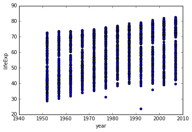
- Plot year vs life expectancy in a scatter plot.
df.plot(x='year',y='lifeExp',kind='scatter')
<matplotlib.axes._subplots.AxesSubplot at 0x7fbac8710b00>
- Plot gdp per capita vs life expectancy in a scatter plot
df.plot(x='gdpPercap',y='lifeExp',kind='scatter', alpha = 0.2, s=50, marker='o')
<matplotlib.axes._subplots.AxesSubplot at 0x7fbac86e87f0>
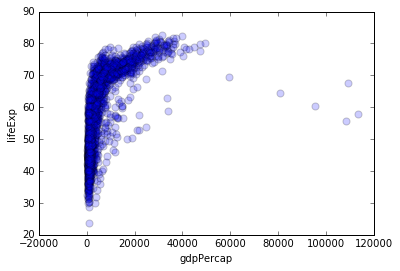
What's going on with those points on the right?
High gdp per capita, yet not particularly high lifeExp. We can use boolean selection to rapidly subset and check them out.
df[df['gdpPercap'] > 55000]
| country | year | pop | continent | lifeExp | gdpPercap | |
|---|---|---|---|---|---|---|
| 852 | Kuwait | 1952 | 160000 | Asia | 55.565 | 108382.35290 |
| 853 | Kuwait | 1957 | 212846 | Asia | 58.033 | 113523.13290 |
| 854 | Kuwait | 1962 | 358266 | Asia | 60.470 | 95458.11176 |
| 855 | Kuwait | 1967 | 575003 | Asia | 64.624 | 80894.88326 |
| 856 | Kuwait | 1972 | 841934 | Asia | 67.712 | 109347.86700 |
| 857 | Kuwait | 1977 | 1140357 | Asia | 69.343 | 59265.47714 |
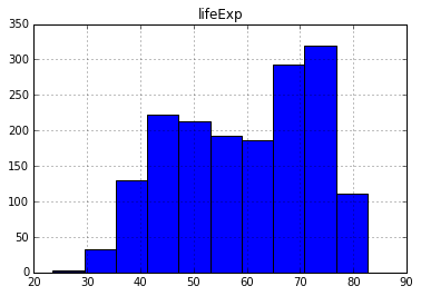
df.hist(column='lifeExp')
array([[<matplotlib.axes._subplots.AxesSubplot object at 0x7fbac5fb3b00>]], dtype=object)
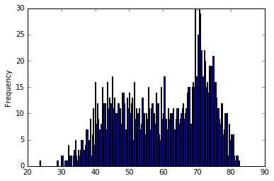
df.lifeExp.plot.hist(bins=200)
<matplotlib.axes._subplots.AxesSubplot at 0x7fbac5fa1a90>
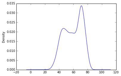
df['lifeExp'].plot(kind='kde')
<matplotlib.axes._subplots.AxesSubplot at 0x7fbac5e5a588>
Exercise
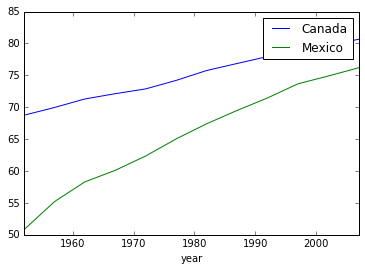
Write a function that will take two countries as an argument and plot the life expectancy vs year for each country on the same axis.
def compare_lifeExp(country1, country2):
    """Plot life expectancy vs year for country1 and country2"""
    ax = plt.subplot()
    for c in [country1,country2]:
        df[df['country']==c].plot(x='year',y='lifeExp', ax=ax)
    plt.legend((country1,country2))
compare_lifeExp('Canada', 'Mexico')
Exercises
Suzy wrote some code to determine which country had the lowest life expectancy in 1982.
What is wrong with her solution?
spec=['country','lifeExp']
df[df['year']==1982][spec].min()
country    Afghanistan
lifeExp         38.445
dtype: object
We can do a quick check to look up Afghanistan's life expectancy in 1982.
df[(df['year']==1982) & (df['country']=='Afghanistan')]
| country | year | pop | continent | lifeExp | gdpPercap | |
|---|---|---|---|---|---|---|
| 6 | Afghanistan | 1982 | 12881816 | Asia | 39.854 | 978.011439 |
This doesnt match with the answer above because the min() function was applied to each column (country and lifeExp).
She should have done this:
df.loc[df[df['year']==1982]['lifeExp'].idxmin()]['country']
'Sierra Leone'
Putting it together:
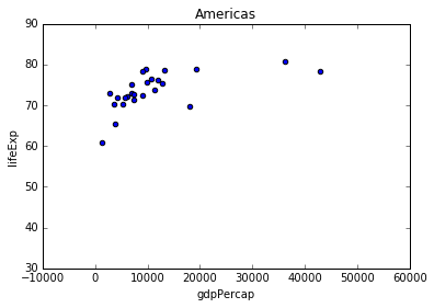
We can use all of these ideas to generate a plot that looks at a subset of the data.
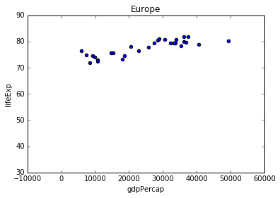
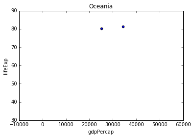
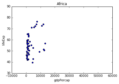
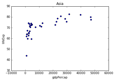
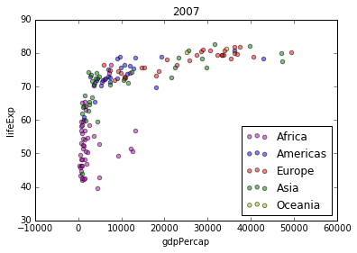
- Plot GDP per capita vs life expectancy in 2007 for each continent.
continents = df.groupby(['continent'])
for continent in continents.groups:
    group = continents.get_group(continent)
    group[group['year']==2007].plot(kind='scatter', x='gdpPercap',
                                    y='lifeExp', title=continent)
    plt.axis([-10000,60000,30,90])
#Example
fig,ax = plt.subplots(1,1)
colours = ['m','b','r','g','y']
for continent, colour in zip(continents.groups, colours):
    group = continents.get_group(continent)
    group[group['year']==2007].plot(kind='scatter',x='gdpPercap',y='lifeExp',label=continent,ax=ax,color=colour,alpha=0.5)
ax.set_title(2007)
plt.legend(loc='lower right')
<matplotlib.legend.Legend at 0x7f5791e0db00>
Exercise
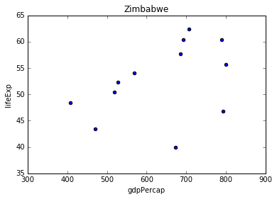
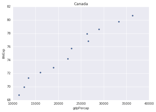
Write a function the takes a country as an argument and plots the life expectancy against GDP per capita for all years in a scatter plot. Also print the year of the minimum/maximum lifeExp and the year of the miniimim/maximum GDP per capita.
def compare_gdp_lifeExp(df,country):
    """ plot GDP per capita against life expectancy for a given country.
    print year of min/max gdp per capita and life expectancy
    """

    sub = df[df['country']==country]
    sub.plot(x='gdpPercap',y='lifeExp',kind='scatter',title=country)

    print('Year of Min/Max GDP per capita')
    print(df.iloc[[sub['gdpPercap'].idxmin(),sub['gdpPercap'].idxmax()]]['year'])
    print('Year of Min/Max life expectancy')
    print(df.iloc[[sub['lifeExp'].idxmin(),sub['lifeExp'].idxmax()]]['year'])
compare_gdp_lifeExp(df,'Zimbabwe')
Year of Min/Max GDP per capita
1692    1952
1696    1972
Name: year, dtype: int64
Year of Min/Max life expectancy
1702    2002
1699    1987
Name: year, dtype: int64
compare_gdp_lifeExp(df,'Canada')
Year of Min/Max GDP per capita
240    1952
251    2007
Name: year, dtype: int64
Year of Min/Max life expectancy
240    1952
251    2007
Name: year, dtype: int64
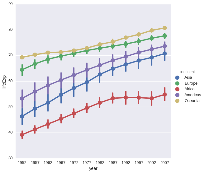
Rapid plotting with seaborn
import seaborn as sns
/home/derek/anaconda2/envs/py3/lib/python3.5/site-packages/IPython/html.py:14: ShimWarning: The `IPython.html` package has been deprecated. You should import from `notebook` instead. `IPython.html.widgets` has moved to `ipywidgets`.
  "`IPython.html.widgets` has moved to `ipywidgets`.", ShimWarning)
df.head()
| country | year | pop | continent | lifeExp | gdpPercap | |
|---|---|---|---|---|---|---|
| 0 | Afghanistan | 1952 | 8425333 | Asia | 28.801 | 779.445314 |
| 1 | Afghanistan | 1957 | 9240934 | Asia | 30.332 | 820.853030 |
| 2 | Afghanistan | 1962 | 10267083 | Asia | 31.997 | 853.100710 |
| 3 | Afghanistan | 1967 | 11537966 | Asia | 34.020 | 836.197138 |
| 4 | Afghanistan | 1972 | 13079460 | Asia | 36.088 | 739.981106 |
sns.set_context("talk")
sns.factorplot(data=df, x='year', y='lifeExp', hue='continent', size=8)
<seaborn.axisgrid.FacetGrid at 0x7f57901cfa20>
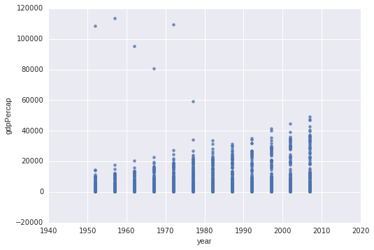
sns.regplot(data=df, x='year', y='gdpPercap', fit_reg=False)
<matplotlib.axes._subplots.AxesSubplot at 0x7fbabf5472b0>
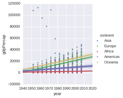
sns.lmplot(data=df, x='year', y='gdpPercap', hue='continent')
<seaborn.axisgrid.FacetGrid at 0x7f579197f710>
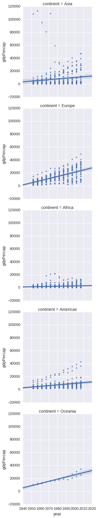
sns.lmplot(data=df, x='year', y='gdpPercap', row='continent')
<seaborn.axisgrid.FacetGrid at 0x7f578da9eb38>
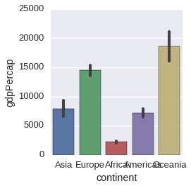
sns.factorplot(data=df, x='continent', y='gdpPercap', kind='bar')
<seaborn.axisgrid.FacetGrid at 0x7f5791ac21d0>
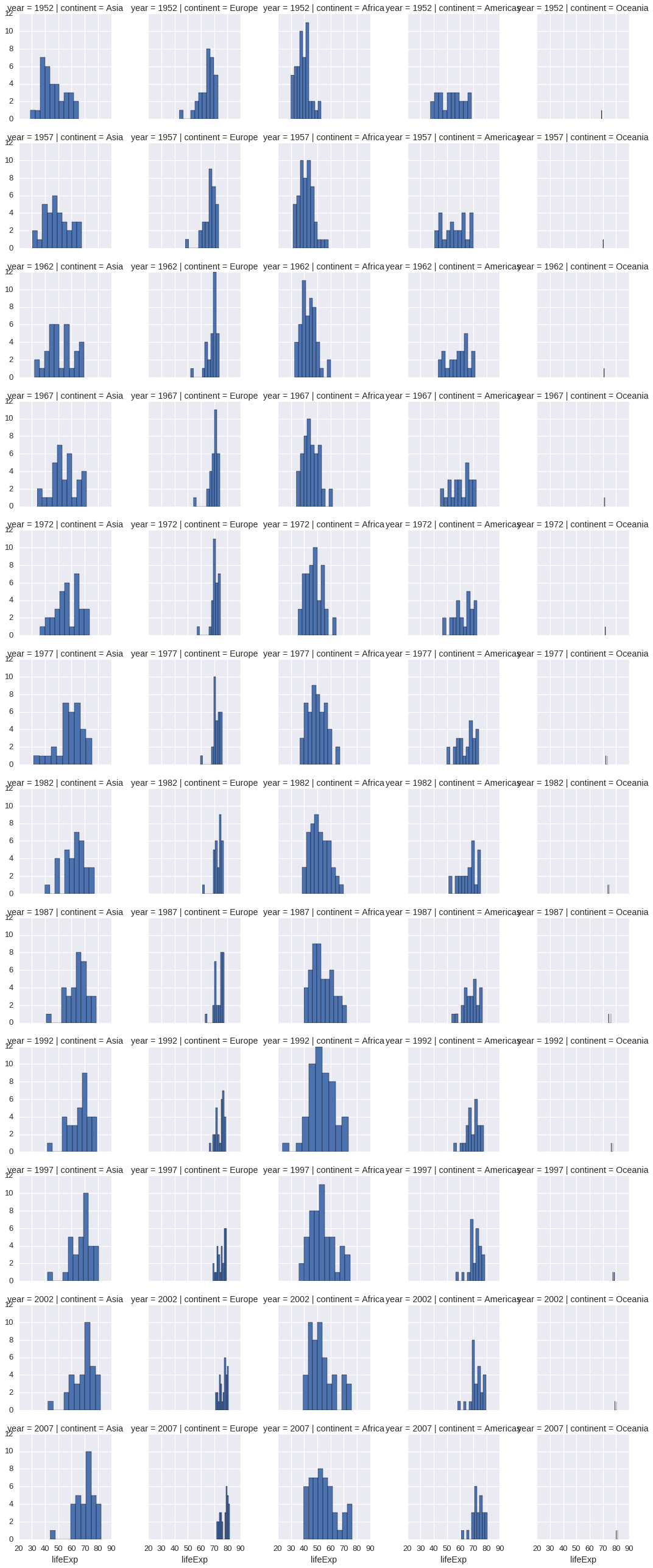
g = sns.FacetGrid(df, col='continent', row='year')
g.map(plt.hist, 'lifeExp')
<seaborn.axisgrid.FacetGrid at 0x7f578d928eb8>